PROGRAM FEATURES |
RESIX 2DI
v4 & IP2DI v4 Click here to download the demonstration program |
|
PROGRAM DESCRIPTION RESIX IP2DI v4 is a finite element forward and inverse modeling program that calculates the IP and resistivity responses of two-dimensional earth models. Inversion can be one of two cell based algorithms or true polygon inversion. The cell based algorithms are also commonly referred to as SMOOTH Models. RESIX 2DI v4 has got the exact same algorithms as RESIX IP2Di v4 but does not support induced polarization (IP) data.
|
Interpex
Smooth Inversion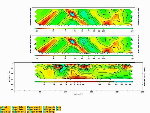 |
Screen capture
shows 2-D pseudosection of the resistivity data at the top, the calculated smooth depth
section at the bottom and the synthetic pseudosection from the depth section in the
middle. Data courtesy of Zonge Engineering.
|
Zonge
Smooth Model Inversion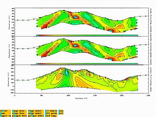
|
Screen capture
shows 2-D pseudosection of the resistivity data at the top, the calculated smooth depth
section at the bottom and the synthetic pseudosection from the depth section in the
middle. The model section presents a 'true' topography section since the topography is incorporated in the model calculation. The model was calculated using the Zonge Smooth model algorithm. Both the data and model sections are draped from topography.
|
Polygon
Model Construct Screen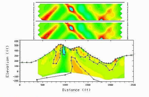
|
Screen capture
shows the polygon model construction screen using the Zonge Smooth Model as a background
to aid in model construction. Polygon models are defined as layers and/or bodies. Any of the vertices and/or body parameters can be set as a FREE parameter in the polygon inversion.
|
Model
Comparison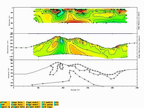
|
Screen capture
shows the Interpex Smooth Model at the top, Zonge Smooth Model in the middle and an
example polygon model at the bottom.
|
| Polygon
Inversion Example Click on the picture to download a AVI file to illustrate the inversion
|
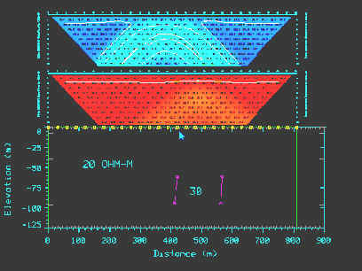
Slide show
demonstrating the POLYGON inversion technique RESIX IP2DI v4 uses. The picture shows the
field data on top with the calculated data from the model shown at the bottom the next
pseudosection. Synthetic data was generated using a box with a resistivity of 10 ohm-m in a halfspace of 100 ohm-m. This data was then transformed to be the field data. To demonstrate the inversion a starting model was assumed to be a box with a resistivity of 30 ohm-m in a halfspace of 30 ohm-m. The box was set up to allow one corner to move freely but the shape of the box was fixed. All resistivity values were also allowed to change in the inversion. It can clearly be seen that the inversion not only changes the position of the box, but also the resistivity values. |
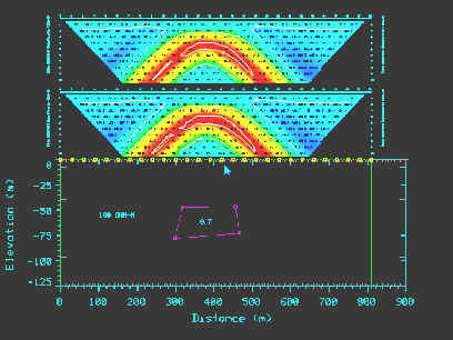
| INVERSION
EXAMPLE Click on the picture to download a AVI file to illustrate the inversion
|
This slide show
is similar to the one above, except that the starting model was a box with all corners
free and all resistivity values free. Again the inversion changes all corners of the body and also the resistivity values to finally produce a model that not only matches the shape of the initial model used to create the synthetic data but also the resistivity values. |
Copyright © 2018 Interpex Limited. All Rights Reserved