![]()
|
![]()
Interpex offers the EMIX MT package to interpret MT, AMT and CSAMT data. EMIX MT performs forward and inverse modeling of layered earth models. Solutions are in terms of either apparent resistivity or apparent resistivity and impedance phase data.
Interpex offers EMIX MT2D to calculate the response of magnetotelluric data to a two dimensional earth model. Results can be presented in terms of profiles, pseudosections or sounding curves.
EMIX MT uses the input impedance concept of J.R. Wait (Theory of Magnetotelluric Fields, National Bureau of Standards, 1962) for forward modeling of the impedance at the surface of the earth. Sounding curves are then converted into apparent resistivity and phase of the impedance in degrees. EMIX MT uses Inman-style ridge regression approach of nonlinear least squares curve fitting for inversion calculations.
EMIX MT is an interactive, graphically oriented, forward and inverse modeling program for interpreting magnetotelluric (MT), audio magnetotelluric (AMT), and controlled source audio magnetotelluric (CSAMT) sounding data in terms of a layered earth (1-D) model. Sounding curves can be entered as a function of period or frequency, and apparent resistivity amplitude data can be interpreted with or without impedance phase data.
Data can be shifted (scaled by a constant) either by using mathematical operators in the Magnetotelluric Data and Error Bars spreadsheet, or by using the Shift curve option while in interactive graphics mode of the INTERPRET command.
Inverse modeling enables you to obtain a model that best fits the data in a least squares sense. This is done using ridge regression (Inman, 1975) to iteratively adjust the parameters of a starting model supplied by the user. Starting models for inversion can have up to 8 layers. You can constrain some of the starting model parameters so the inversion will not adjust them. Constants can be applied by fixing (or freezing) a parameter, or by imposing limits on a parameter. Parameters can be resistivity + thickness of layers, or resistivity + depth to bottom of layers. If phase data are present, each layer has an additional parameter.
Smooth modeling enables you to automatically interpret MT amplitude and impedance phase sounding data in terms of a smooth model with up to 19 layers. The model depths are logarithmically spaced and are generated from a minimum and maximum depth. The minimum and maximum depth can be user-specified or can be automatically generated. Model resistivities are normally initialized to the best fit homogeneous half-space resistivity. Inversion can be carried out in either interactive or batch mode, using ridge regression or William of Occam's smooth model concept. Results can be plotted, printed, listed on the screen, or written to an ASCII file for use by user-supplied or third-party software.
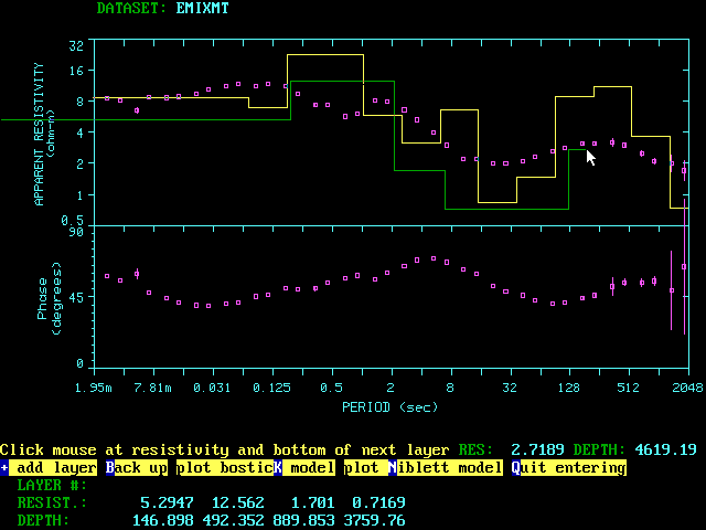
Interactive graphics interpretation screen showing the Phase and Apparent Resistivity data. Model construction is done using the mouse. The Bostic model is displayed as a guide for model construction.
Equivalence analysis enables you to generate a set of equivalent layered models, that is, alternative models that fit the data nearly as well as the best-fit model, but differ from this model. Equivalence analysis also indicates the allowable range of each of the model parameters.
Results from forward or inverse modeling can be directed to a printer and/or plotter for report-ready, hard-copy output. Results can also be saved in a binary random access disk file for later retrieval. Inverse modeling can be carried out in an unattended batch mode.
EMIX MT provides several options to present the observed data, the theoretical (forward) data, and the geological model section used to calculate the forward response. A plate-style format can graphically present all this information; or, each type of information can be presented individually on a dot matrix printer, a laser printer, or a pen plotter. You can also print the data and model section in a tabulated, paginated form directly to a text printer.
EMIX MT allows for the specification of a profile distance and TE, TM or No specified mode. This allows EMIX MT2D to access the EMIX MT database and assign a TE and a TM mode sounding to a station at the specified location along the profile.
EMIX MT can also handle controlled source data taken with a grounded wire. The grounded wire is assumed to be a dipole and the receiver is assumed to be oriented so that the electric field receiver is parallel to the source wire.
![]()
EMIX MT2D is an interactive, graphically oriented forward modeling program for interpreting magnetotelluric sounding data taken along a profile in terms of a 2-D earth model. Sounding curves are entered into EMIX MT and assigned as TE or TM mode. EMIX MT2D accesses the EMIX MT database and allows the 1-D interpretations (layered or smooth models) to be displayed during 2-D model building or editing. The 2-D modeled sounding curves, the local 1-D sounding curves or the data can be displayed.
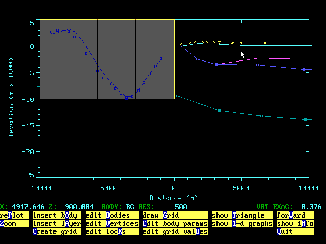
Interactive model construct screen from EMIX MT2D showing 1-D sounding data obtained from EMIX MT database in pop-up window.
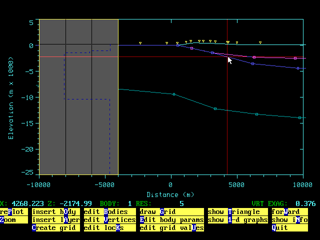
Interactive model construct screen from EMIX MT2D showing 1-D model results obtained from EMIX MT database in pop-up window.
EMIX MT 2D can also be used to generate synthetic data from 2-D models without having field data.
Model creation is done by drawing the geological cross-section as layers or bodies. Bodies are closed polygons while layers are entered from left to right and automatically closed at infinity. EMIX MT 2D automatically generates the finite element mesh using the resistivities of the bodies and layers and parameters editable by the user. The resulting grid can be edited by the user, either numerically or graphically.
On screen interactive model editing allows the user to change, delete, insert bodies and to zoom the display. The resistivity values and topography can easily be edited. The program calculates results for the TE mode, TM mode or both.
EMIX MT2D determines the starting dimensions of the finite element grid automatically from the number of stations and the station spacing. The package automatically creates a near optimum grid based on the topographic relief, skin depths, and horizontal resistivity contrasts. It assigns a very high resistivity value for air.
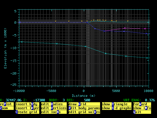
Interactive model construction in EMIX MT2D showing grid and model. Grid elements can be added, deleted and split using the mouse
Up to 50 stations can be placed at any location along the profile line. Importation of field data in EMIX MT format can generate station locations automatically or assign field stations to existing EMIX MT2D stations.
Calculations are carried out using a finite element method similar to that described by Wannamaker and Stodt (Geophysical Journal of the Royal Astronomical Society 88, 1987). Both conventional and extended (EMS or XMS) memory is used in the finite element solution.
Several options allow for field data or 1-D inversion results (from EMIX MT) to be displayed during 2-D model construction and editing. TE,TM field data and/or 2-D model results can be displayed by simply pointing at a station on the 2-D cross-section display. The local 1-D model results can also be displayed. Alternatively, the results of 1-D modeling for TE, TM and/or Occam's inversion (Smooth Model Results) can be displayed over the 2-D model as an aid in model construction or editing. The user has control over which mode and which data/models are displayed.
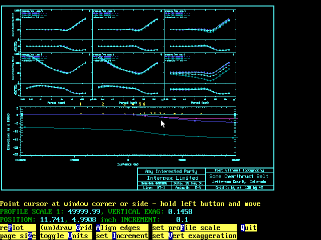
Sample interactive plate configuration showing the model and MT Soundings calculated at several points along the profile.
EMIX MT2D provides several options to display the results of modeling. Single stations can be displayed with field curves and local 1-D results as desired.
Modeling results can be displayed in pseudosection or profile form, along with annotated model cross section, if desired. Multiple soundings can be presented together with the model cross section on a single large plot. Field data can be shown with the 2-D model results.
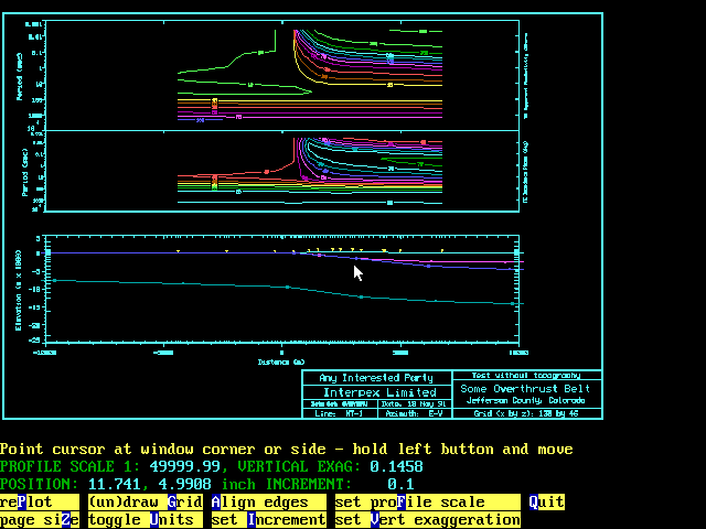
View Plate screen showing data and model. Interactive plate editing allows the user to set page size, resize graphic plot elements and set vertical exaggeration.
Features and maximum parameters: