Interpex offers three software tools that interpret resistivity and induced polarization soundings in terms of 1 dimensional models. These tools belong to the RESIX family of software. Use any one of these software packages to produce forward and inverse models of resistivity data, or induced polarization data, or both.
![]()
For forward modeling, all RESIX family programs use an Anderson-style adaptive linear digital filter for most common arrays to provide you with resistivity contrasts of up to 10,000 to 1. For stable results for inversion, all programs use the Inman-style ridge regression approach of nonlinear least squares curve fitting.
RESIX is an interactive, graphically oriented, forward and inverse modeling program for interpreting resistivity sounding data in terms of a layered earth (1-D) model. Sounding curves can be entered as a function of a for Wenner or pole-pole soundings, AB/2 for Schlumberger soundings, R for dipole soundings or N for dipole-dipole or pole-dipole soundings.
Sounding curves values are entered as apparent resistivity as a function of spacing. Forward modeling enables you to calculate a synthetic resistivity sounding curve for a model with up to ten plane layers. Resistivity sounding curves are calculated using linear filters.
Shifting of data with overlapping curve segments is handled automatically by shifting the synthetic curve to match the offsets between segments in the data. This is done by assuming the data for the longest spacings is correct, and shifting segments at shorter spacings to meet the data at longer spacings. Alternatively, you can shift the data curve itself to meet either the longest or shortest spacing segment. This can be done either automatically, or manually in the interactive graphics mode using the Shift Segments option.
Masking of data is achieved in the interactive graphics interpretation module by pointing and clicking on data points. These points can be unmasked or deleted according to the users needs. Masked points do not influence the error or inversion calculations.
Interactive model input via the mouse allows the user to see changes in the calculated curve as he enters the model graphically. Graphic entities of the plate output may also be resized and positioned using the mouse.
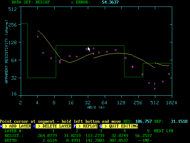
Screen from RESIX showing interactive model input using the mouse.
Inverse modeling allows you to obtain a model that best fits the data in a least squares sense, using ridge regression to interactively adjust the starting model parameters. You can constrain some of the starting model parameters so the inversion will not adjust them. Starting models for inversion can have up to 8 layers. Forward models can have as many as 10 layers. Constants can be applied by fixing (or freezing) a parameter, or by imposing limits on a parameter. Parameters can be resistivity / thickness of layers, or resistivity / depth to bottom of layers.
Results from forward or inverse modeling can be directed to a printer or plotter for report-ready, hard-copy output. Results can also be saved in a binary random access disk file for later retrieval. Inverse modeling can be carried out in an unattended batch mode.
RESIX provides several options to present the observed data, the theoretical (forward) data, and the geo-electrical model section used to calculate the forward response. This information can be graphically presented individually on a dot matrix printer, a laser printer, or a pen plotter. You can also print the data and model section in a tabulated, paginated form directly to a text printer.
Data storage is handled by a new data base file format which holds up to 200 data sets (or sounding curves). The size of the file depends on the number of sounding curves it contains.
RESIX PLUS has all the features of RESIX with the following additions.
Sounding curves can be entered as apparent resistivity versus spacing; or, the voltage, current, and electrode spacings for both current and potential electrodes can be entered on the worksheet. The worksheet calculates apparent resistivities as you enter the data, using formulas that account for the finite electrode spacings.
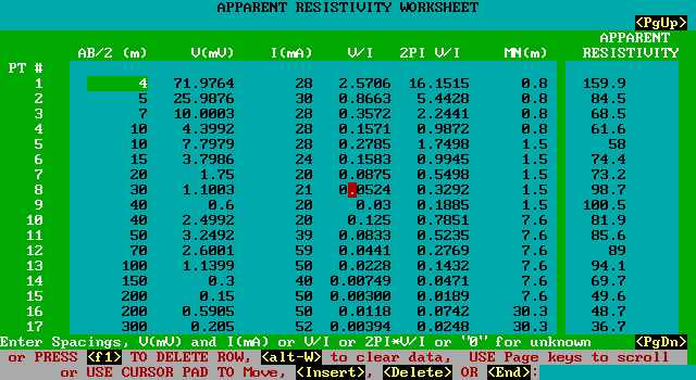
Data Edit Worksheet from RESIX Plus.
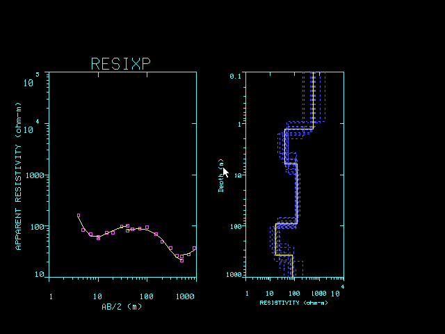
Direct inversion allows you to estimate the layered model directly from the data curve, without having to manually construct the number of layers and layer resistivity and thickness. Extension of the input data curve for short and long electrode spacings, and curve resampling and transformation, are done automatically and are transparent.
Smooth modeling enables you to automatically interpret resistivity sounding data in terms of a smooth model with up to 19 layers. The model depths are logarithmically spaced and are determined from a minimum and maximum depth. The depth range can be user-specified or automatically generated. Model resistivities are normally initialized to the average apparent resistivity. Inversion can be carried out in either interactive or batch mode, using ridge regression or William of Occam's smooth model concept. Results can be plotted, printed, listed on the screen or written to an ASCII file for use by user-supplied or third-party software.
Equivalence analysis allows you to generate a set of equivalent models, (that is, alternative models that fit the data nearly as well as the best-fit model, but differ from this model). Equivalence analysis also indicates the allowable range of model parameters.
Plot of equivalent models from RESIX Plus.
The MODEL SUITE command enables you to construct a collection of forward models by specifying one or more different values for a parameter. You can also generate new electrode spacings. This enables you to see the results of a specific change to the original model.
RESIX PLUS offers the user the capability to enter Offset Wenner Sounding resistances in to the Offset Wenner worksheet or read them from Campus Geophysical Instruments ASCII files thereby replacing the OFFIX and BOSSIX programs.
RESIX IP is an interactive, graphically oriented, forward and inverse modeling program for interpreting induced polarization (IP) and resistivity sounding data in terms of a layered earth (1-D) model.
RESIX IP has all the features of RESIX PLUS with the following exceptions where the program was adapted to incorporate Induced Polarization (IP) data.
Sounding curves can be entered as a function of a for Wenner or pole-pole soundings, AB/2 for Schlumberger soundings, R for dipole soundings or N for dipole-dipole or pole-dipole soundings. Apparent resistivity data can be interpreted with or without apparent polarization data.
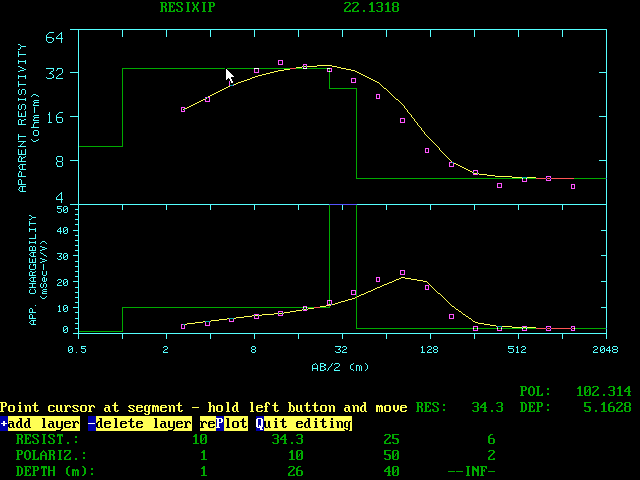
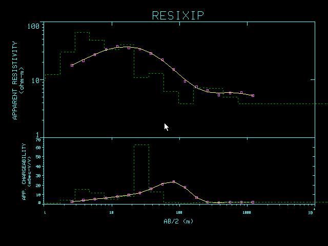
Interactive modeling in RESIX IP.
Forward modeling enables you to calculate synthetic IP/resistivity sounding curves for a model with up to 10 plane layers. IP readings can be entered in units of mSec-V/V or in percent frequency effect (PFE).
Inverse modeling enables you to obtain a model that best fits the data in a least squares sense. Starting models for inversion can have up to 7 layers if both resistivity and polarization parameters are included, or up to 10 layers if only resistivity parameters are included. Forward models can have as many as 10 layers. Constraints can be applied by fixing (or freezing) a parameter, or by imposing limits on a parameter. Parameters can be resistivity + thickness of layers, or resistivity + depth to bottom of layers. If IP data are present, each layer has an additional parameter, either chargeability or PFE, according to the choice of data type.
Equivalence analysis functions similarly to equivalence analysis in RESIX PLUS, but RESIX IP generates equivalent models for both resistivity and IP models.
The MODEL SUITE command functions similarly to the MODEL SUITE command in RESIX PLUS, but RESIX IP generates suites of models for both resistivity and IP data.
Screen from RESIX IP showing model suites and calculated results for a range of resistivity values visible.
Smooth modeling functions similarly to smooth modeling in RESIX PLUS, but RESIX IP generates smooth models for both resistivity and IP data.
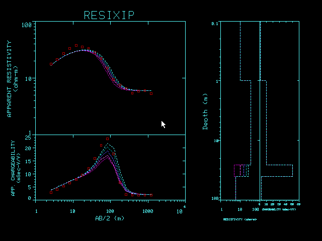
Screen from RESIX IP showing smooth model plot on same plot axis as resistivity and IP data.