|
 |
Interpex is a software company dedicated to the production of high quality
software for the processing, interpretation and display of geophysical data.
|
|
P.O. Box 839 •
Golden • Colorado • 80402 • USA
e-mail: info@interpex.com |
This site does not use cookies. We do not collect any personal information on
this site.
Home
Marine EM
Seismic Processing Custom Development DOS
Support
Do Not Program Your
Key!
Windows 11

IX1D-mTEM
1D Marine
Sounding Inversion
IX1DmTEM is a
1-D Marine electromagnetic sounding inversion program with the following features:
-
Supports TEM Inline E, crossline H, broadside E, joint
inline E with crossline H and (coming soon)
multiple offset E-field soundings.
-
Supports step current on, step current off or current
impulse.
-
Supports
Frequency domain inline E and broadside E data.
-
Supports isotropic or anisotropic resistivity models.
- IX1D has the capability to read in a
resistivity well log from a flat ASCII file and the user can
interactively reduce the log to several discreet layers by fitting
straight line segments to the cumulative conductance in the log. The
resulting model can be copied to the model in the current data set
for further modeling. The log can be read in as an isotropic or
anisotropic (vertical and horizontal) resistivity. For
anisotropic models, the cumulative resistance is also
displayed and can be used to create layer boundaries.
Features include:
-
Creation of data by spreadsheet entry
or copy/paste from another spreadsheet.
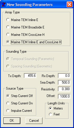
Data Type and Parameter Dialog Box

DC
Resistivity Voltage/Current Data Entry Dialog Box
-
Import of data
or models from flat ASCII files.
-
Models
are entered from the keyboard or copy/pasted from a spreadsheet as either Depth models or Layer Thickness.
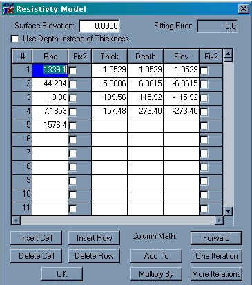
Model Entry Dialog Box
-
Layer boundary elevations are
shown and calculated relative to surface and keyboard
elevations.
-
The Model Entry dialog box
allows for dynamic column and row manipulations to make
model entry more convenient. Fix Flags allow the user to fix
parameters for the inversion calculations. Either the layer
thickness (or depth) and/or the resistivity can be fixed in
the inversion process.
-
Forward and inverse model
calculations can be carried out using buttons on the model
entry dialog. Models can be inverted using either the layer
depth or layer thickness.
-
Graphics are presented as the
Sounding data on the left hand side with the model on the
right hand side. Interactive property sheets allows for user
configuration of displayed data.
-
Menu commands and toolbar
buttons are available for estimating a smooth model or
analyzing equivalence of the layered model.
-
Supports
model suite generation for isotropic and anisotropic
models, allowing variation of single layer resistivity,
thickness or depth, source receiver offset, sea depth or
resistivity, transmitter depth or a second model can be
faded in. Existing data can be displayed with curve
suite. Time base can be from existing data or generated
from parameters.
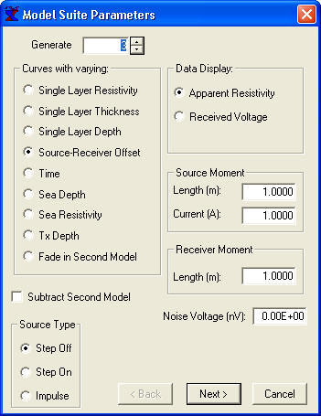
Model Suite
Dialog
-
Smooth models are generated
by starting with as many layers as the user desires. Thicknesses
are automatically generated from the min and max depths specified and the model begins
with a homogeneous earth (all layers set to the average resistivity
found in the data). Inversion can be Ridge Regression or Occam's
inversion.
-
The sounding
window display can be set to show the layered model, smooth
model, equivalence analysis or any combination of these
three.
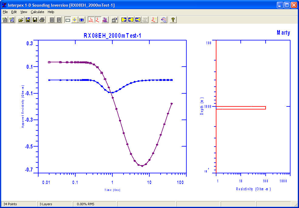
Sounding Window Graphics Screen
-
The model and data plots can
be zoomed by dragging the mouse across the display with the left button
depressed. This feature can be switched on and off by clicking on the
Zoom menu command in the View menu or by clicking on the Zoom tool bar
icon.
-
Axis labels as well as axis
sizes can be edited under View Properties. Grid lines, including major
and minor, for the Data and Model axes can be switched on and off under
the View Grid menu subchoices. Axes can be auto-scaled from the model
and data by selecting the View Unzoom menu command.
-
Data, Layered models and
Smooth models can be exported to ASCII files.
-
Graphics can be exported as
DXF, CGM or WMF file formats.
-
Tool bar buttons are
provided for the most-used menu commands, including New Sounding or
Model, Open and Import data, Save, Print, Edit Data or Model, Zoom
status, Unzoom, model display selection, Forward, Inverse and
Equivalence Analysis calculations, and Estimation of Smooth
models.
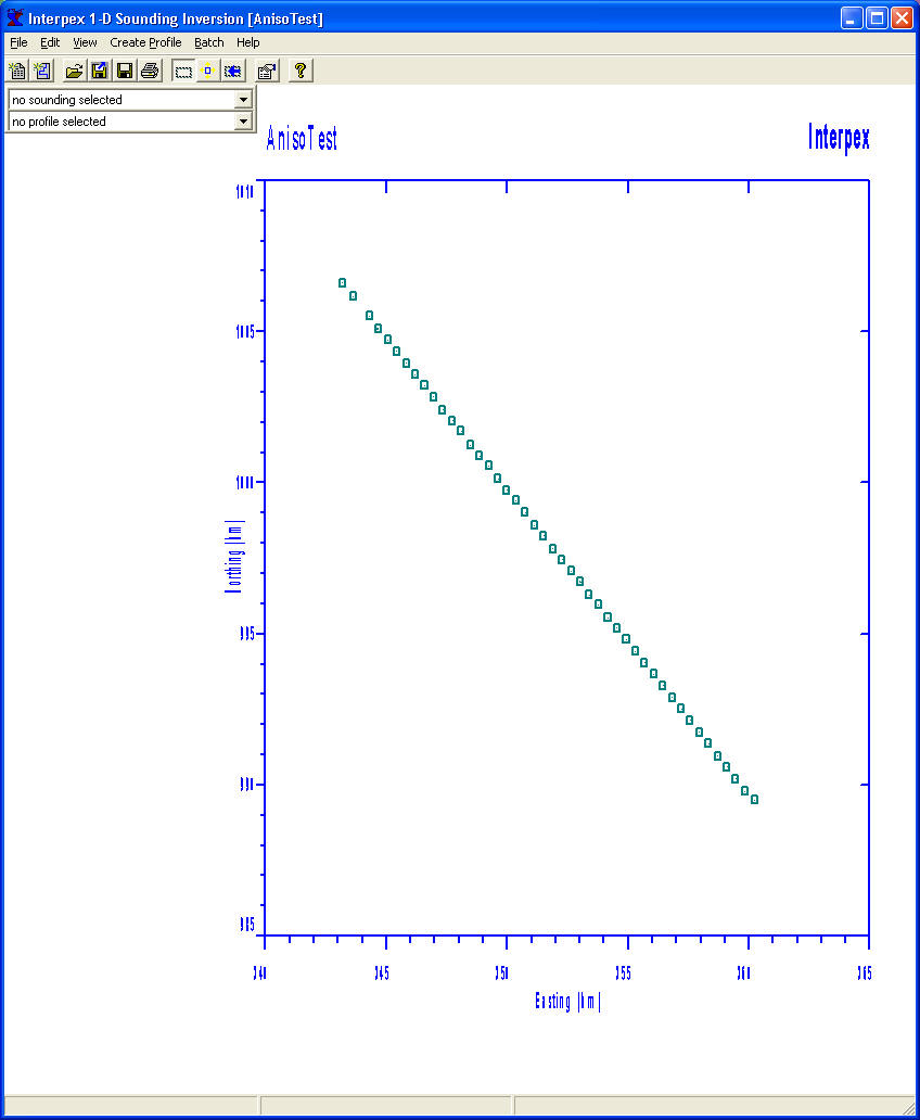
Display of Soundings
in Map Coordinates.
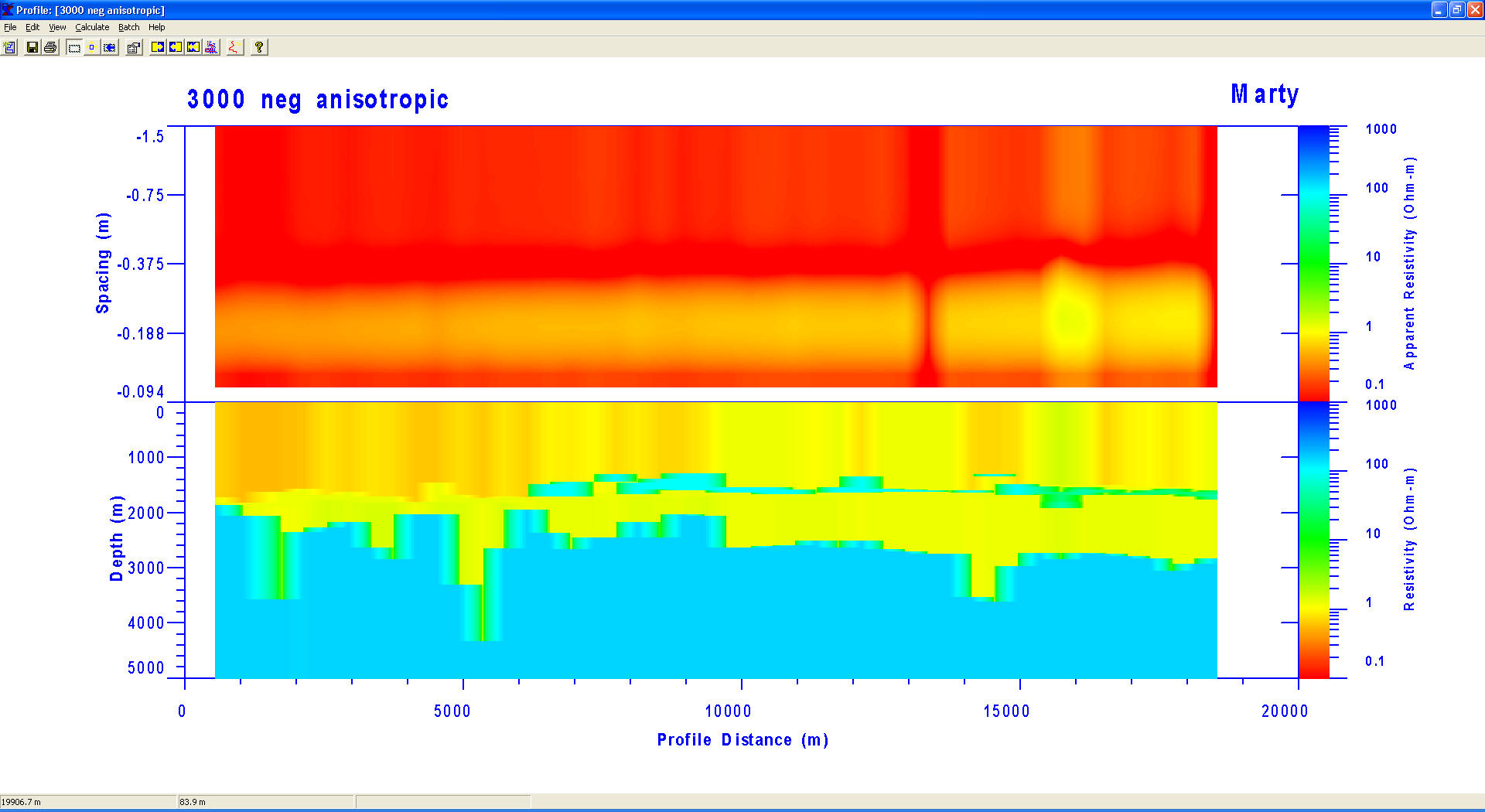
Display of inline E Data with data displayed as
pseudosection and smooth model displayed as a
colored section
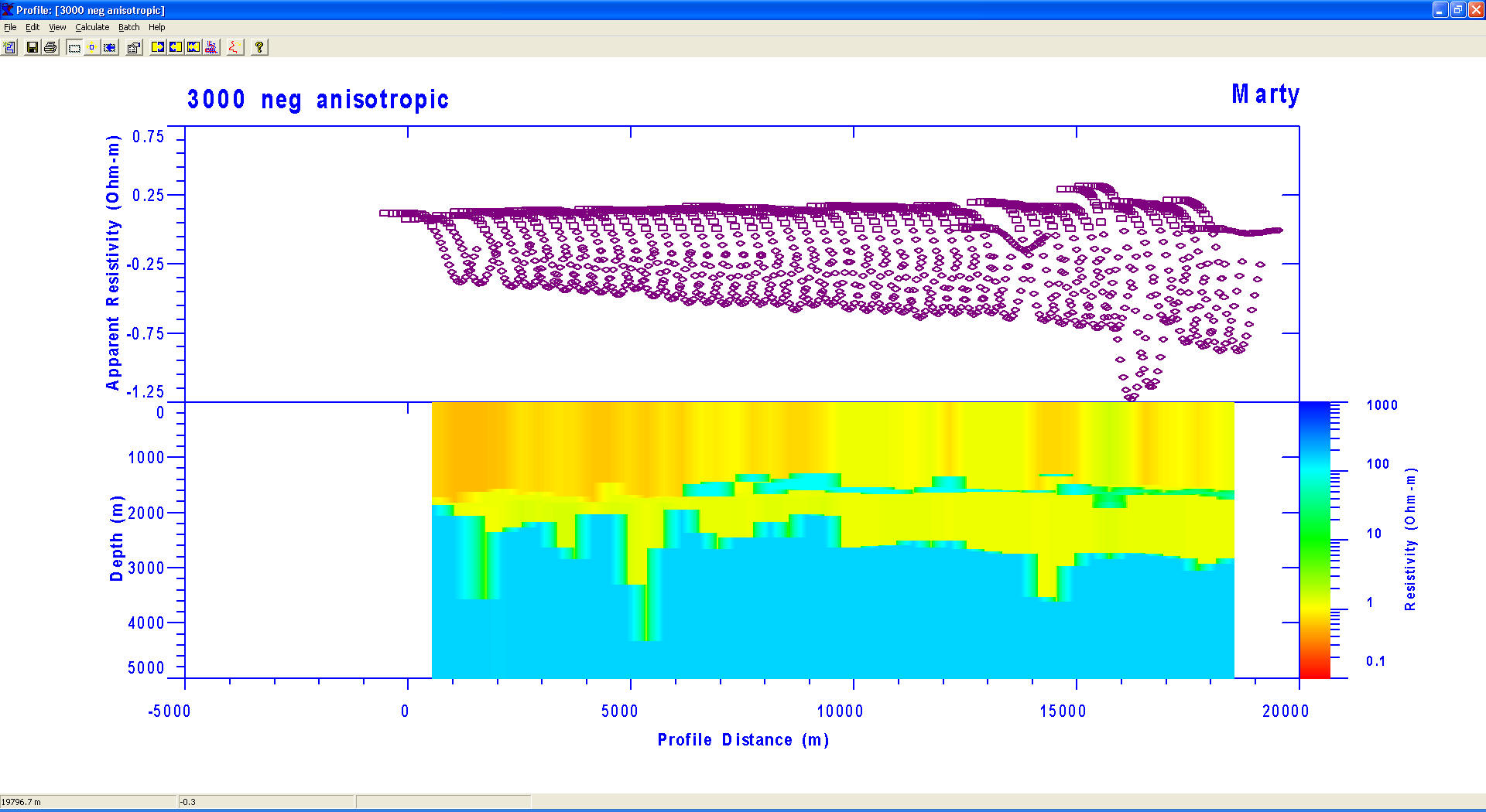
Display of
Inline E Data with apparent resistivity data displayed as
curves on a Zaborovsky plot and smooth model displayed as a
colored section.
-
Forward modeling, inverse
modeling, smooth model estimation and equivalence analysis can be
carried out individually or in batch or pseudo-batch mode.
-
Profiles and soundings can
be selected by name or by point and click at a map location. Soundings
on a profile can be selected by point and click on a profile location.
-
A model can be copied to the
model clipboard and then back to an individual sounding, all soundings
on a profile or to every sounding in the database.
-
Creation of data
by spreadsheet entry or copy/paste from another spreadsheet.
-
Import of data or models from flat ASCII files
-
Models are
entered from the keyboard as either Depth models or Layer
Thickness or copy/paste from another spreadsheet.
- Layer boundary elevations are shown
and calculated relative to surface, sea bottom or keyboard elevations.
-
The Model Entry dialog box allows
for dynamic column and row manipulations to make model entry more
convenient.
-
Fix Flags allow the user to fix
parameters for the inversion calculations. Either the layer thickness (or depth)
and/or the resistivity can be fixed in the inversion process.
-
Forward and inverse model
calculations can be carried out using buttons on the model entry dialog.
Models can be inverted using either the layer depth or layer thickness.
-
Graphics in the Sounding
Window are presented as the
Sounding data on the left hand side with the model on the right hand side.
Interactive property sheets allows for user configuration of displayed
data.
-
Menu commands and toolbar
buttons are available for estimating a
smooth model or analyzing equivalence of the layered model. These appear
on the sounding window and on the profile window. Using the command from
the profile window executes a pseudo-batch operation where each sounding
along the profile is processed in turn.
-
View Properties are
available for the sounding window, the profile window and the map
window. Axes in the map window are never vertically exaggerated. View
Properties for the profile window allows for control of the
resistivity color fill range and parameters.
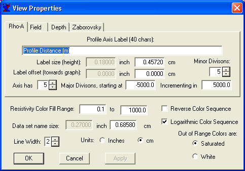
Axes Label Properties
-
When smooth model estimation
is started from the Profile window, smooth models are generated
by starting with the same starting model for each sounding along the
profile. The user selects the number of layers, the starting and ending
depths and the starting resistivity. The model begins
with a homogeneous earth (all layers set to the specified resistivity). Inversion can be Ridge Regression or Occam's
inversion.
-
The display in the sounding
window can be set to
show the layered model, smooth model, equivalence analysis or any
combination of these three. For DC Resistivity data, the model(s) can also be shown on the same
graph as the data, in which case the spacing axis doubles as a depth
axis. For colored section displays, the smooth model section is
displayed if View/Smooth is selected; otherwise the layered model is
displayed.
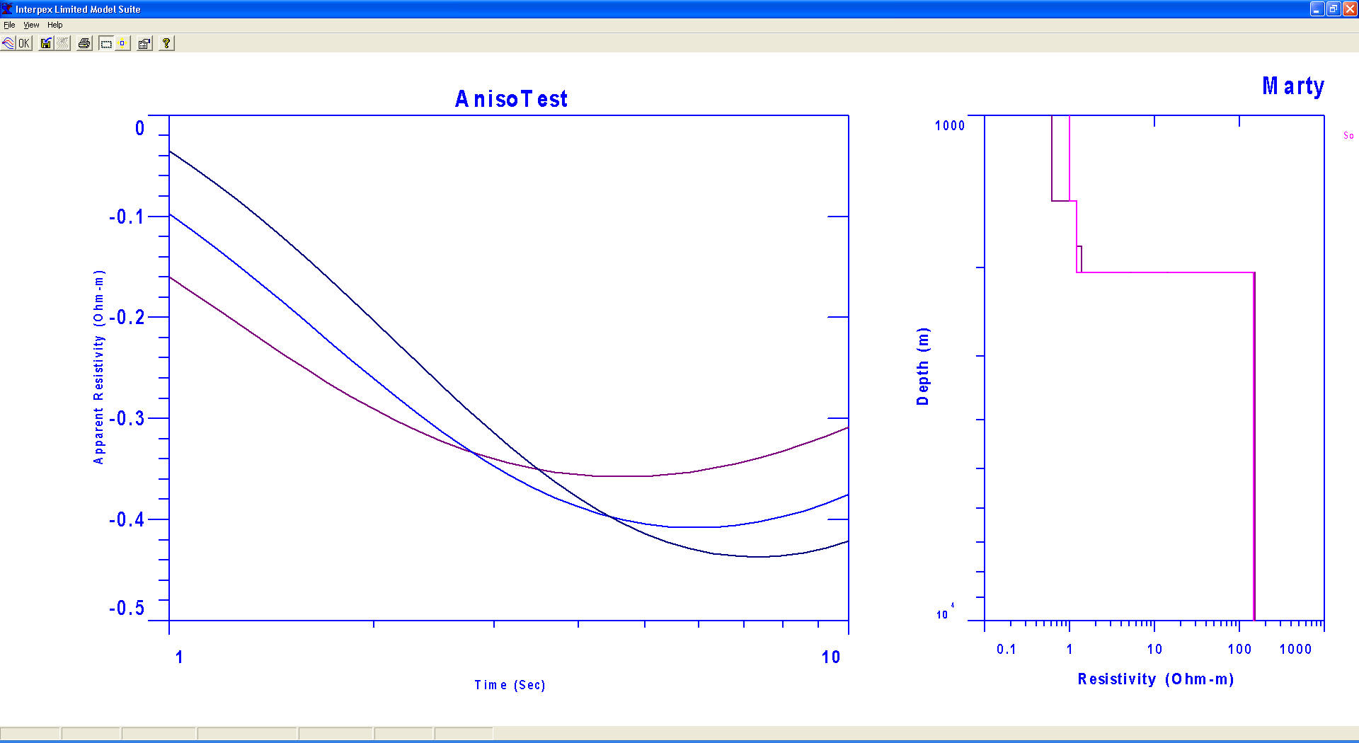
Model Suite
window showing 3 curves for varying offsets with the same
anisotropic model.
-
For MT data, the Bostick and
Niblett inversions can also be shown.
-
Soundings can be selected
for display from the map window if no profile is displayed. Or they can
be selected from the Profile Window.
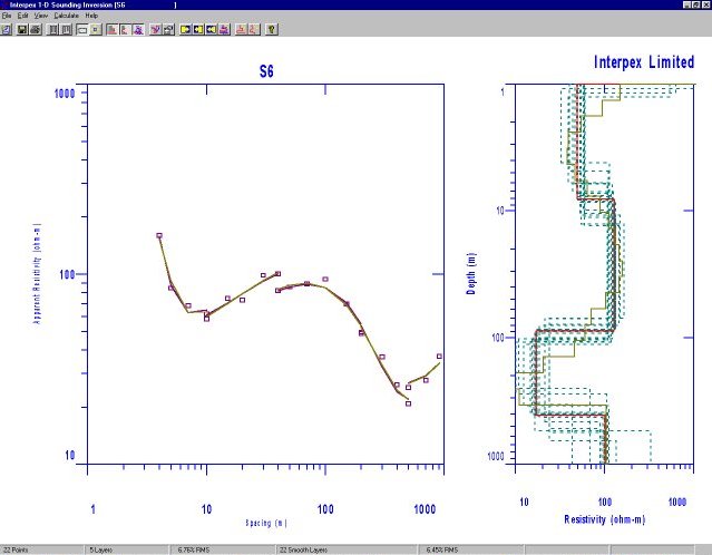
Sounding Display Window showing smooth model, layered model and equivalence
analysis.
-
The model and data plots can
be zoomed by dragging the mouse across the display with the left button
depressed. This feature can be switched on and off by clicking on the
Zoom menu command in the View menu or by clicking on the Zoom tool bar
icon.
-
Axis labels as well as axis
sizes can be edited under View Properties. Grid lines, including major
and minor, for the Data and Model axes can be switched on and off under
the View Grid menu subchoices. Axes can be auto-scaled from the model
and data by selecting the View Unzoom menu command.
-
Data, Layered models and
Smooth models can be exported to ASCII files.
-
Graphics can be exported as
DXF, CGM or WMF file formats.
-
Tool bar buttons are
provided for the most-used menu commands, including New Sounding or
Model, Open and Import data, Save, Print, Edit Data or Model, Zoom
status, Unzoom, model display selection, Forward, Inverse and
Equivalence Analysis calculations, and Estimation of Layered or Smooth
models.
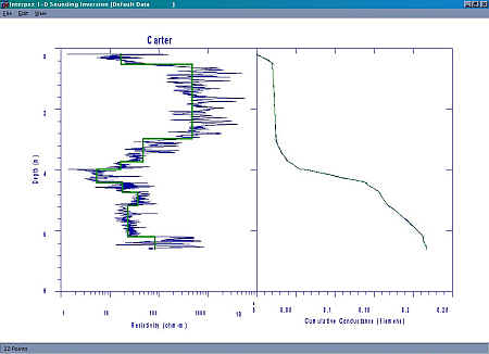
Resistivity Well log shown
with layered model decomposition
Licensing and Distribution
IX1D
version 3 is distributed as copy-protected software. The software can be
downloaded and it works fully only with the demo data supplied. The license allows for a 30-day evaluation period.
After the evaluation you are required to purchase the package in order to
continue using it. Purchase price is US$999.00 for DC, IP, MT, Frequency EM and EM
Conductivity capabilities. The price for for TEM is an US
$3,499.00. Both licenses are offered with your choice of USB or Parallel key.
Licensed Versions
Licensed
users can obtain e-mail support by sending requests for assistance, bug fixes
and feature enhancements to info@interpex.com
Please include the serial number, version number and attach the
files with which you are having problems to your e-mail request.
The
newest version can be downloaded from this website and will work with your
licensed hardware key. Updates are free if you download them from our web site.
|
